A fact table is the one which consists of the measurements, metrics or facts of business process. These measurable facts are used to know the business value and to forecast the future business. 

The different types of facts:

Additive:

Additive facts are facts that can be summed up through all of the dimensions in the fact table. A sales fact is a good example for additive fact.

Semi-Additive: 

Semi-additive facts are facts that can be summed up for some of the dimensions in the fact table, but not the others.
Eg: Daily balances fact can be summed up through the customers dimension but not through the time dimension.

Non-Additive: 

Non-additive facts are facts that cannot be summed up for any of the dimensions present in the fact table. 
Eg: Facts which have percentages, ratios calculated.

Factless Fact Table:

In the real world, it is possible to have a fact table that contains no measures or facts. These tables are called "Factless Fact tables".

Eg: A fact table which has only product key and date key is a factless fact. There are no measures in this table. But still you can get the number products sold over a period of time.

TRUNCATE

• TRUNCATE is a DDL command
• TRUNCATE is executed using a table lock and whole table is locked for remove all records.
• We cannot use Where clause with TRUNCATE.
• TRUNCATE removes all rows from a table.
• Minimal logging in transaction log, so it is performance wise faster.
• TRUNCATE TABLE removes the data by deallocating the data pages used to store the table data and records only the page deallocations in the transaction log.
• Identify column is reset to its seed value if table contains any identity column.
• To use Truncate on a table you need at least ALTER permission on the table.
• Truncate uses the less transaction space than Delete statement.
• Truncate cannot be used with indexed views.

DELETE

• DELETE is a DML command.
• DELETE is executed using a row lock, each row in the table is locked for deletion.
• We can use where clause with DELETE to filter & delete specific records.
• The DELETE command is used to remove rows from a table based on WHERE condition.
• It maintain the log, so it slower than TRUNCATE.
• The DELETE statement removes rows one at a time and records an entry in the transaction log for each deleted row.
• Identity of column keep DELETE retain the identity.
• To use Delete you need DELETE permission on the table.
• Delete uses the more transaction space than Truncate statement.
• Delete can be used with indexed views.

DROP

• The DROP command removes a table from the database.
• All the tables' rows, indexes and privileges will also be removed.
• No DML triggers will be fired.
• The operation cannot be rolled back.
• DROP and TRUNCATE are DDL commands, whereas DELETE is a DML command.
• DELETE operations can be rolled back (undone), while DROP and TRUNCATE operations cannot be rolled back.

What is a Dimension Table: 
 A table which consists of the attributes about the facts is called a Dimension Table.
Dimensions store the textual descriptions of the business. It helps to measure the facts.

The different types of dimension tables:

1. Conformed Dimension: It mean the exact Dimension Table liked with every possible fact table to which they are joined.  Eg: The date dimension table connected to the sales facts is identical to the date dimension connected to the inventory facts.
2. Junk Dimension: A junk dimension is a collection of random transactional codes flags and/or text attributes that are unrelated to any particular dimension. The junk dimension is simply a structure that provides a convenient place to store the junk attributes. Eg: Assume that we have a gender dimension and marital status dimension. In the fact table we need to maintain two keys referring to these dimensions. Instead of that create a junk dimension which has all the combinations of gender and marital status (cross join gender and marital status table and create a junk table). Now we can maintain only one key in the fact table.
3. Degenerated Dimension: A degenerate dimension is a dimension which is derived from the fact table and doesn't have its own dimension table.  Eg: A transactional code in a fact table.
4. Role-playing dimension: Dimensions which are often used for multiple purposes within the same database are called role-playing dimensions. For example, a date dimension can be used for “date of sale", as well as "date of delivery", or "date of hire"

Fast growing dimension or SCD Type 4:

In slowly changing dimensions the dimension tables tend to grow slowly. Example: Location attribute of a customer changes very rarely. 

However the salary band of a customer is likely to change every year. These type of attributes causes the customer dimension table to grow rapidly and we need Fast Growing Dimension or SCD Type 4.

In SCD type 4 a junk dimension or a small dimension table with all the possible values of the rapid growing attributes of the dimension are maintained and a  dimension key of the new table should be maintained in the fact table. This way we can handle the rapid changes in the dimension table. 

Example : Dimension attributes of customer

C_Id
Name
Location
Age_band
Salary_band

The new tables are 

Table name : customer
C_Id
Name
Location

Table name: customer_mini
M_id
Age_band
Salary_band

Fact table:
Id
C_Id
M_Id
----

SCD type 2 stores the entire history the data in the dimension table. With type 2 we can store unlimited history in the dimension table. In type 2, you can store the data in three different ways. They are

1. Versioning
2. Flagging
3. Effective Date

SCD Type 2 Versioning: In versioning method, a sequence number is used to represent the change. The latest sequence number always represents the current row and the previous sequence numbers represents the past data.

Example a customer (Deb) moves from Cuttack to Bangalore and the version number will be incremented. The dimension table will look as below

SCD Type 2 Flagging: In flagging method, a flag column is created in the dimension table. The current record will have the flag value as 1 and the previous records will have the flag as 0.

SCD Type 2 Effective Date: In Effective Date method, the period of the change is tracked using the start_date and end_date columns in the dimension table.

Slowly changing dimensions are the dimensions in which the data changes slowly, rather than changing regularly on a time basis.

For example, you may have a customer dimension in a retail domain. Let say the customer is in India and every month he does some shopping. Now creating the sales report for the customers is easy. Now assume that the customer is transferred to United States and he does shopping there. How to record such a change in your customer dimension?

You could sum or average the sales done by the customers. In this case you won't get the exact comparison of the sales done by the customers. As the customer salary is increased after the transfer, he/she might do more shopping in United States compared to in India. If you sum the total sales, then the sales done by the customer might look stronger even if it is good. You can create a second customer record and treat the transferred customer as the new customer. However this will create problems too.

Handling these issues involves SCD management methodologies which referred to as below

1. SCD Type 1
2. SCD Type 2
3. SCD Type 3

COMPOSITE PARTITONING:

Composite partitioning partitions data using the range method, and within each partition, subpartitions it using the hash method. Composite partitions are ideal for both historical data and striping, and provide improved manageability of range partitioning and data placement, as well as the parallelism advantages of hash partitioning.

When creating composite partitions, you specify the following:

Partitioning method: range
Partitioning column(s)
Partition descriptions identifying partition bounds
Subpartitioning method: hash
Subpartitioning column(s)
Number of subpartitions for each partition or descriptions of subpartitions
The following statement creates a composite-partitioned table. In this example, three range partitions are created, each containing eight subpartitions. Because the subpartitions are not named, system generated names are assigned, but the

STORE IN clause distributes them across the 4 specified tablespaces (tab1, …,tab4).

CREATE TABLE PRODUCTS (partno NUMBER,
description VARCHAR(32),
costprice NUMBER)
PARTITION BY RANGE (partno)
SUBPARTITION BY HASH (description)
SUBPARTITIONS 8 STORE IN (tab1, tab2, tab3, tab4)
(PARTITION p1 VALUES LESS THAN (100),
PARTITION p2 VALUES LESS THAN (200),
PARTITION p3 VALUES LESS THAN (MAXVALUE));

List Partitioning: 

• It is used when it's required to have explicit control over how rows map to partitions. 
• It can have list  of discrete values for the partitioning column in the description for each partition. 
• This is different from range partitioning, where a range of values is associated with a partition, and from hash partitioning, where the user has no control of the row to Partition mapping.
• List partitioning allows unordered and unrelated sets of data to be grouped and organised together very naturally.
• 
  

Syntax for list partitioning:

 Create table customers (custcode number (5),
Name varchar2 (20),
Addr varchar2 (10,2),
City varchar2 (20),
Bal number (10, 2))
Partition by list (city),
Partition north_India values (‘DELHI’,’CHANDIGARH’),
Partition east_India values (‘KOLKOTA’,’PATNA’),
Partition south_India values (‘HYDERABAD’,’BANGALORE’,
’CHENNAI’),
Partition west India values (‘BOMBAY’,’GOA’);


If a row is inserted in the above table then oracle maps the value of city column and whichever partition list matches the city column the row is stored in that partition.

Hash partitioning: 

• It is used  if data does not easily lend itself to range partitioning, but you would like to partition for Performance and manageability reasons. 
• It provides a method of evenly distributing data across a Specified number of partitions. 
• Rows are mapped into partitions based on a hash value of the partitioning key

 Syntax for Hash partitioning

CREATE TABLE products
(PRDNO NUMBER,
Description VARCHAR2 (60))
PARTITION BY HASH (partno)
PARTITIONS 4
STORE IN (tab1, tab2, tab3, tab4);

Above example creates a hash-partitioned table, The partitioning column is PRDNO, four partitions are created and assigned system generated names, and they are placed in four named tablespaces (tab1, tab2, …).

Oracle Partitioning by Range:  This type of partitioning is useful when dealing with data that has logical ranges into which it can be distributed; for example, value of year. 

Performance is best when the data evenly distributes across the range.

In Oracle Partition allows tables, indexes, and index-organized tables to be subdivided into smaller pieces, enabling these database objects to be managed and accessed at a finer level of granularity. These enhance the query performance. 

In Oracle a Table can be partition by below ways:

1. Range Partitioning
2. Hash Partitioning
3. List Partitioning
4. Composite Partitioning

Bitmapped indexes:

Oracle  bitmap index is generally used for columns of low Cardinality (Columns with lots of duplicate values) . Bitmap index structures is made of a two-dimensional array.

• This two-dimensional array represents each value within the index multiplied by the number of rows in the table. 
• During query Oracle decompresses the bitmap into the RAM data buffers so it can be rapidly scanned for matching values. 
• These matching values are delivered to Oracle in the form of a Row-ID list, and these Row-ID values may directly access the required information.

A bitmap and a btree indexes are used to retrieve rows faster than a full-table scan.  

Below are the basic differences between b-tree and bitmap indexes :

1:  Syntax of bitmap and a B-tree indexes:  

• The bitmap index includes the "bitmap" keyword.  
• The btree index does not say "bitmap"

2: Cardinality differences:  

• The bitmap index is generally for low cardinality columns (Columns with duplicate values )
• while b-tree indexes are best for high cardinality columns.

3: Internal structure differences:  

• A B-tree index has index nodes (based on data block size), it like a tree form

• A bitmap index looks like this, a two-dimensional array with zero and one (bit) values

Kimball vs. Inmon Data Warehouse Architectures, It's quite an interesting comparison between the two models.
 
Each Model have it's own importance and usage.

1. Kimball Data Warehouse Architecture
2. Inmon Data Warehouse Architecture

Degenerative Dimension :

According to Ralph Kimball, in a data warehouse, a degenerate dimension is a dimension key in the fact table that does not have its own dimension table, because all the interesting attributes have been placed in analytic dimensions. The term "degenerate dimension" was originated by Ralph Kimball.

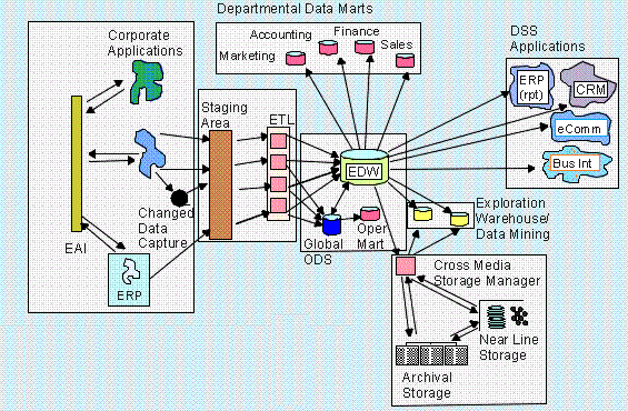
Corporate Information Factory or Bill Inmon Data Warehouse Architecture is mostly based on EDW (Enterprise Data Warehouse ) concept.

Bill Inmon Data Warehouse Architecture

1. Corporate Applications such as operational systems or transaction systems, that are used to support business. Transaction systems are used to collect data from business transactions such as sales, marketing, material managements…..etc and stored those data in various forms including relational data, hierarchical data or even spreadsheets. In Inmon’s architecture, transaction systems are also called source systems that provide data to the data warehouse.
2. ETL Processes. To bring data from the transaction system, a process called ETL is used. ETL stands for extract, transform and load. ETL process consolidates data, transform it into a specific standard format and load it into a single repository called enterprise data warehouse, or EDW. ETL processes can run as a batch process periodically or a transaction-based for near real-time data. ETL process is referred as data integration or data services.
3. Enterprise data warehouse is a central element in the Inmon’s data warehouse architecture. As Inmon’s data warehouse definition, enterprise data warehouse is an integrated repository of atomic data. Data in the enterprise data warehouse is captured at a very lowest level of detail. Data in the enterprise data warehouse is stored in relational database and uses third normal database design.
4. Data marts are departmental views of information with subject oriented data. Data marts take data from enterprise data warehouse. Aggregations can take place when data brings from enterprise data warehouse to data marts. Data marts use dimensional design, therefore, the data in the data marts is ready for analysis. It is important to note that all the external applications or reporting tools or business intelligence tools query data from data marts instead of enterprise data warehouse directly.

Ralph Kimball data warehouse architecture which is also widely known as dimensional data warehouse architecture.

Ralph Kimball Data Warehouse Architecture

Below are some of the silent feature of Ralph Kimball Data Warehouse Architecture

1. Transaction applications are the operational systems created to capture business transactions. The data of transaction system usually stored in relational databases (DBs) or Files (such as flat File or Spreadsheets). Those transaction systems are source systems of the data warehouse in Ralph Kimball data warehouse architecture.
2. Data is brought from transaction system in variety forms using the ETL processes (Tools Such as Informatica or Data Stage or Oracle Data Integrator ). ETL stands for Extract,Transform , & Load. Usually data in different formats is standardized and converted into a single format that ready to load into the data warehouse.
3. Dimensional data warehouse is the center of data warehouse architecture. The dimensional data warehouse contains enterprise data in a very granular format. Where as Bill Inmon’s data warehouse architecture uses ER modeling, the dimensional data warehouse is designed using dimensional modeling technique. It means dimensional data warehouse consists of star schema schema model or cubes. The analytic systems or reporting tools can access data  from these dimensional data warehouse directly.
4. Data mart. In this architecture, data mart concept is just a logical distinction. The data mart is a subject area within the dimensional data warehouse.

OBIEE 11g Factless fact Table

 Factless Fact ? What does it mean, what's the use ?

Here's the Answer a factless fact table is a fact table that does not have any measures. These fact tables are non additive fact in nature.

In Short a Factless Fact has below attributes :

1. Contains no Measures
2. Non Additive in nature

Use of Factless Fact: 

Events sometime are modeled as a fact table containing a series of keys for each dimensions involved in the event. So these event tables have no numeric (Measures) facts associated with them and hence are called factless fact tables.

Example :

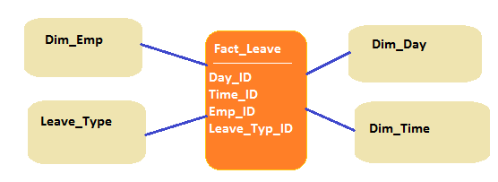
  The above fact is designed to capture the leaves taken by an employee, So whenever an employee takes leave a record is inserted into the Fact Table with the help of dimension keys.

Using the fact Fact_Leave some of the Below analysis can be done

• Leave Count by Employee
• Type of Leave utilization
• Detials of Employee Taking leaves